

It’s CITY CYCLING time – some of you may even be involved in your municipality – a good opportunity to have a look on the OpenStreetMap (OSM) cycling ways in our city Heidelberg.
Welcome to part 8 of our how to become ohsome blog post series. This time we will show you how to set up a more complex filter with several OR and AND combinations for the ohsome API to get the length of the mapped cycling ways in OSM. Like in part 4 of our series, we will again show you in a Jupyter Notebook how you can use Python to make this nice complex ohsome query and visualization in one go.
The idea is to analyse the mapped cycle ways in Heidelberg in OSM. Therefore we need to have a look on how cycling infrastructure is mapped in OSM. To set up the filter, we want to know which tags do we need to extract all the cycle lanes, ways and roads. There is more than one way to tag cycle ways, lanes or paths in OSM, described for example on this OSM wiki page. Instead of requesting every possible tag by itself, all combinations of tags that can be used to define a cycle way within OSM can be requested at once using our new filter parameter. This also prevents ways being counted twice, which might have several of these tags associated with them.
Our tag combination is based on Hochmair, Zielstra, and Neis’s paper Assessing the completeness of bicycle trails and designated lane features in OpenStreetMap for the United States and Europe. In their study they explored the cycling features in the United States and Europe. We take their filter combination and extend it with tags of the German cycling infrastructure mapping methods listed on the corresponding OSM wiki page. After a pre-query for each of the tag combinations we found out that for some of them no data was available for the region of Heidelberg, so we excluded them. As a result we got a filter that consists of 25 different tag combinations.
The final filter looks like following:
type:way and ((bicycle=use_sidepath) or(cycleway=opposite and oneway:bicycle=no) or(sidewalk:right:bicycle=yes) or(cycleway:right=shared_lane) or(cycleway:left=track) or(cycleway:right=track) or(highway=track and bicycle=designated and motor_vehicle=no) or(highway=path and bicycle=yes) or(highway=path and (bicycle=designated or bicycle=official)) or(highway=service and (bicycle=designated or motor_vehicle=no)) or(highway=pedestrian and (bicycle=yes or bicycle=official)) or(highway=footway and (bicycle=yes or bicycle=official)) or(highway=cycleway) or(cycleway in (lane, opposite_lane, shared_busway, track, opposite_track)) or(cycleway:left in (lane, shared_busway)) or(cycleway:right in (lane, shared_busway)) or(cycleway:both=lane) or(bicycle_road=yes and (motor_vehicle=no or bicycle=designated)) or(cyclestreet=yes))
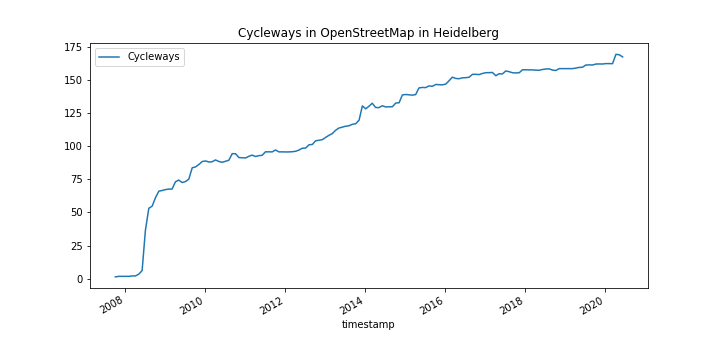
The official number given by the city of Heidelberg of cycle path network is about 480 kilometers, which is almost 3 times as many kilometers as there are in OSM. The difference may be due to the fact that there are some side roads that have an extra lane, others do not, or that sometimes a appropriate tag is really missing in OSM. In addition, in the explanation of the cycle road map for Heidelberg, the city’s network includes normal roads which have signposted cycle routes running through to neighbouring communities such as Leimen, Eppelheim, Dossenheim and Edingen.
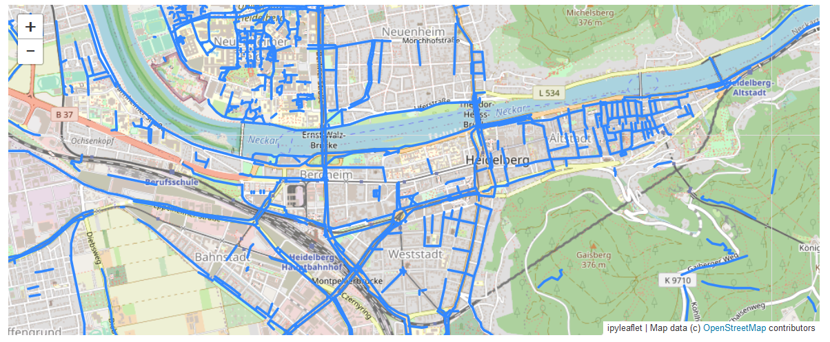
We can also take a spatial look at the current expansion of the cycle path network. For this we use the same filter as above but in the data extraction endpoint of the ohsome API. A snippet of the request can be found here.
So if you are interested in the mapped cycling infrastructure in OSM in your city, just change the bounding box geojson in the code and find it out ![]() . The complete Jupyter Notebook with all the code and explanations can be found here.
. The complete Jupyter Notebook with all the code and explanations can be found here.
If you want to know more about our ohsome framework, don’t hesitate to reach out to us via info(at)heigit.org or contact any member of our team directly. Stay ohsome and happy cycling!
Information on the ohsome OpenStreetMap History Data Analytics Platform and more examples of how to use the ohsome API can be found here:
- ohsome general idea
- ohsome general architecture
- the whole “how to become ohsome” tutorials series
- filter subpage of our new documentation page
- Scientific article on OSHDB
- OSHDB and ohsome API git repositories
- For some recent work that has been accomplished using this framework see for example Analyzing the spatio-temporal patterns and impacts of large-scale data production events in OpenStreetMap In: Minghini, M., Grinberger, A.Y., Juhász, L., Yeboah, G., Mooney, P. (Eds.). Proc. of the Academic Track at the State of the Map 2019, 9-10. Heidelberg
or Auer, M.; Eckle, M.; Fendrich, S.; Griesbaum, L.; Kowatsch, F.; Marx, S.; Raifer, M.; Schott, M.; Troilo, R.; Zipf, A. (2018): Towards Using the Potential of OpenStreetMap History for Disaster Activation Monitoring. ISCRAM 2018. Rochester. NY. US.
or Wu, Zhaoyan, Li, Hao, & Zipf, Alexander. (2020). From Historical OpenStreetMap data to customized training samples for geospatial machine learning. In proceedings of the Academic Track at the State of the Map 2020 Online Conference, July 4-5 2020. DOI: http://doi.org/10.5281/zenodo.3923040
or Ludwig, C., Fendrich, S., Zipf, A. (2020 accepted): Regional Variations of Context-based AssociationRules in OpenStreetMap. Transactions in GIS DOI: 10.1111/tgis.12694