
Welcome to part 2 of the #ohsome street network analysis. If you haven’t read the first part yet, you can do so following this link. As promised, this week we are performing a simple tag completeness analysis, where we are looking at the ratio between streets that have the maxspeed tag added and those which are not bearing this specific tag. At the end of this blogpost we display an overall ranking, where we crown the winning “region of the month”.
Data:
Like last time you can get the spatial data set used as the area of interest in our requests via this website. Again, you will have to send POST requests to get the desired dataset from our global ohsome API instance for which you’ll find the cURL commands (and more!) in a snippet here.
The endpoint used for this weeks analysis is: /elements/length/ratio/groupBy/boundary which gives out the calculated ratio between, in this case, the length of streets with a tagged maxspeed and those that do not have that information added. Since it is grouped by boundary you will get a dataset which is subdivided by each city.
The parameters defined for this request are:
format = csv
filter = type:way and highway in (primary,secondary,tertiary,motorway)
filter2 = type:way and highway in (primary,secondary,tertiary,motorway) and maxspeed=*
time = 2010-12-01/2020-12-01/P1M
Unlike the analysis in part one, this weeks focus is on the main roads, which is why the filter conditions for the highway key are less broad.
Data exploration:
In the graphic below you can see the development of the ratio of the length of roads, which have a maxspeed tag added in comparison to the total length of said roads. A ratio of 1 would indicate that all of the analyzed roads have a maxspeed tag.
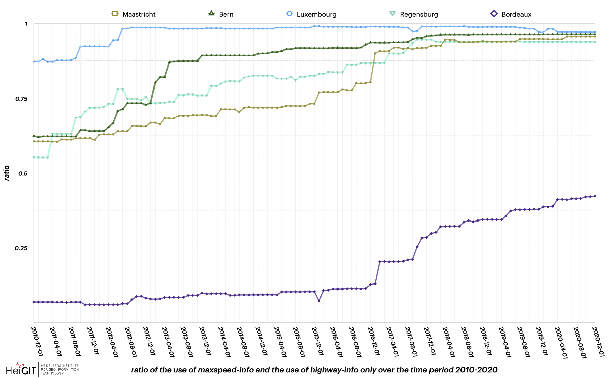
Again there appears to be almost no direct connection between certain data imports and sudden developments within the dataset. The most obvious part is Bordeaux with very low ratio values in comparison to the other cities, which have different starting values but are aligning in a rather close range around the beginning of 2018. Furthermore notable is the increasing converging tendencies of each citys individual maxspeed-info and general highway-info.
Especially for Luxembourg those values are approaching early, which leads to the overall seemingly stable values. It also has the overall highest ratio values from start to end. One can see a phase of several strong jumps/increases until July 2016 which is followed by more or less stable values. Since the values were really high in the beginning already, Luxembourg does not score that well in terms of ∆- and p%-values.
For Bern there is almost no development until September 2011 followed by a phase of several stronger increases until May 2013 for which no explanation connected to user counts or data imports could be found. Subsequent to a few more minor jumps and an overall slow increase, the Bern dataset reaches stability at around December 2017/January 2018.
The Maastricht ratio development shows a steady, positive trend until December 2016 which is followed by a very strong increase between December 2016 and January 2017, to be precise an increase by a ratio of ~0.096. This sudden jump in Winter 2016/17 seems to be happening for Bordeaux too, so these two might be connected. However, we couldn’t find an explanation for the sudden ratio increases.
When looking at the Regensburg data it displays a strong, ‚jumpy‘ increase until June 2012 followed by a decreasing movement until about January of the following year. This is most likely connected to new mapped roads that do not have the maxspeed tag initially. The same assumption can be applied to other datasets showing this pattern
The Bordeaux dataset individually shows a strong ratio increase, which starts in November 2016 whilst before the trend was rather moderately positive. Since there appear to be no connections to user counts or data imports whatsoever, the question as to why Bordeaux has such low ratio values remains. Taking a look at certain conventions seems to be a logical step, but in regard of information to the maxspeed tag such as the OSM wiki, one gets an insight on the speed limits given in the countries where the examined cities are. For France, there seems to be a clear connection between the highway tag and the allowed maxspeed. Other countries though, like the Netherlands and Switzerland, have conventions similar to France, but this does not seem to have an impact on the availability of the maxspeed tag, at least when looking at the analyzed regions
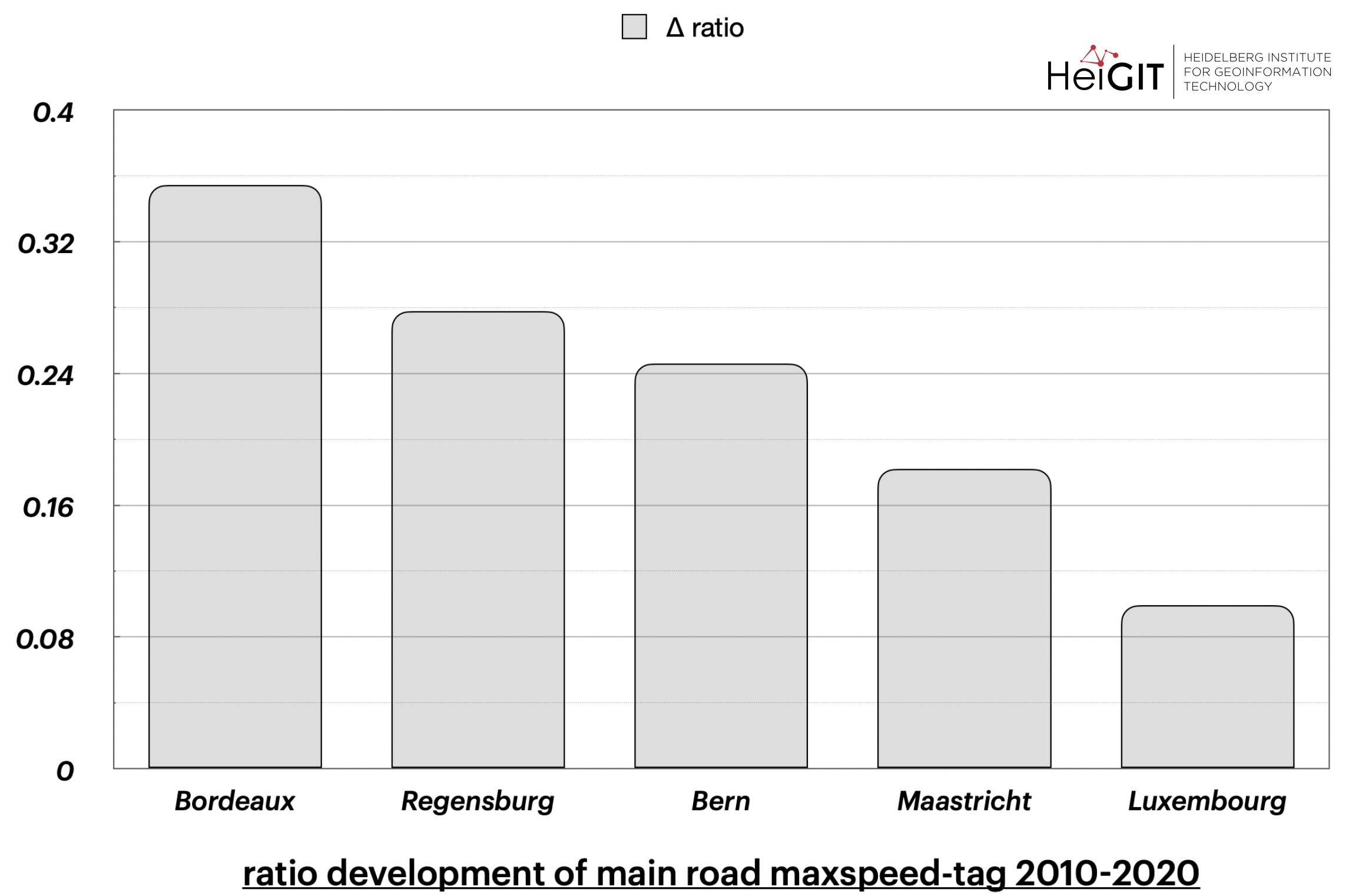
Below you can see the percentage development of each city’s ratio* (top graphic) as well as the ∆ ratio values showing the absolute changes (bottom graphic).
*minus Bordeaux because the values were so high they distorted the graphic; you can still find it enclosed in the snippet

Users:
As in the first part you can get the user data for this request too, but this time you’ll have to split it in 2 individual requests in case you would like to compare both of them. Following graphic displays the maximum (top end), minimum (low end) and mean (horizontal line) user count of the main-road info.
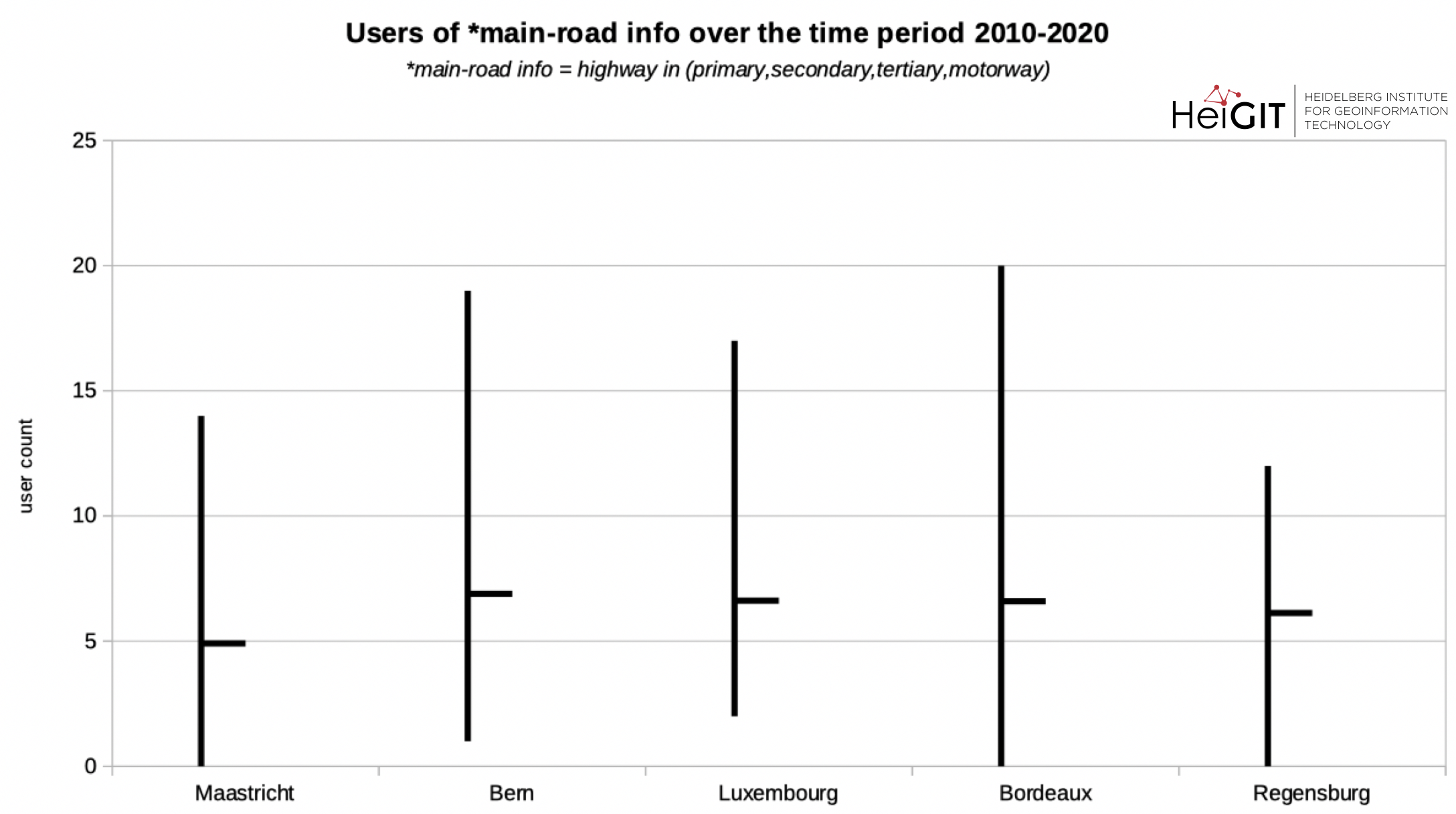
In general, there appears to be only little connection between the the ratio development and the user counts. The minimum amount of users for Maastricht is reached in June 2012, which also happens to be the end of an increase in the ratio values within the Maastricht data set. The maximum is reached in August 2017, a month that is followed by a decrease in the ratio dataset, which might be a reflection of the unusually high amount of users. The assumption is that roads were mapped in this period, but not all of them had an associated maxspeed tag, hence the lower ratio. The Luxembourg ratio-maximum is reached in July 2019 and is also followed by the beginning of the last decreasing phase in such. This too might be a reflection of the unusually high user count at this point of time.
For Regensburg, the peak is reached in October 2012, which is followed by a decreasing ratio trend similar to the third maximum in May 2014, which is the last month of an increasing phase. For Bordeaux, as well as Bern, there appears to be no connection at all between the user counts and the course of the ratio time series.
Now we are coming to the rankings of this weeks analysis, which look as follows:
Ranking by latest ratio values:
- Luxembourg
- Bern
- Maastricht
- Regensburg
- Bordeaux
Ranking by ∆ ratio-values:
- Bordeaux
- Regensburg
- Bern
- Maastricht
- Luxembourg
Region of the month:
The region of the month is identified with the help of a scoring system that is split into two parts: The first part is the sum of the overall ranking of the latest values that are represented in the first ranking table here and in the table that we’ve shown at the end of last weeks blog post using a weighting of 1. The second part uses the individual development of each city. It is comprised of the sum of the p%- together with the arithmetic mean values of each city using a weighting of 0.5. Let’s take a look on how the score of Luxembourg was computed:
ranking of latest ratio values: 4th and 1st
ranking of p% values: 1st and 5th
ranking of mean values (see snippet): 4th and 1st
final ranking computation: 4+1+0.5*(1+5+4+1)=10.5
With that scoring system we get the following final ranking:
- Luxembourg
- Bordeaux
- Bern
- Maastricht
- Regensburg
So there we have it: Our region of the month is Luxembourg with Bordeaux coming in second and Bern 3rd, followed by Maastricht on the 4th place. Regensburg did unfortunately not manage to get a higher ranking and remains on the last spot. If you want to perform such statistical analysis yourself using one of our tools, don’t hesitate to contact us via ohsome(at)heigit.org.
Background info: the aim of the ohsome OpenStreetMap History Data Analytics Platform is to make OpenStreetMap’s full-history data more easily accessible for various kinds of OSM data analytics tasks, such as data quality analysis, on a regional, country-wide, or global scale. The ohsome API is one of its components, providing free and easy access to some of the functionalities of the ohsome platform via HTTP requests. Some intro can be found here:
-
ohsome general idea
-
ohsome general architecture
-
how to become ohsome blog series
-
how spatial joins queries work in the OpenStreetMap History Database OSHDB