
Welcome back to another #ohsome blog post written by our awesome student assistent Sarah! This time we will look at the completeness of railway network data of one specific city in OpenStreetMap, as well as its development. For this we looked at the city of Prague and its completeness of the operator tag. Furthermore, you’ll get to see the development of the railway network data of Prague in an animation (and can even learn how to make one yourself!). In case you haven’t read the last ohsome region of the month blogposts, you can find part 1 here & part 2 here.
Data:
As usual you will have to think of the boundaries you’re going to set in your analysis. For this you again have to get your hands on a spatial data set with the boundaries of Prague (e.g. from here) in the GeoJSON format. The dataset of interest in regard of our railway network analysis can be accessed by sending a request to the ohsome API.
Requests:
For the visualization of the evolution we decided to use the operator tag as indicator, so we can display the ratio of railway network with that information given, as well as the point in time where this information startet to get added and the point in time when it reached its maximum value. We created a snippet with the final cURL POST requests, as well as the parameter text files and further information here.
You will have to use two endpoints for getting the needed data. One is /elements/length/ratio for the part where you want to look at the ratio development over the years and the other one is /elementsFullHistory/geometry so you can access and visualize the whole evolution of railway network data (as given in the filter). With this data extraction request you’ll get all the changes to the railway network within your given timeframe, as well as the duration of validity of these changes, which comes in handy when working on the evolution animation.
Analytical Visualization:
endpoint: /elements/length/ratio
timestamp: 2009-01-01/2021-01-01/P1M
filter: type:way and railway in (rail,light_rail,subway,tram,narrow_gauge) and operator=*
Evolution Visualization:
endpoint: /elementsFullHistory/geometry
timestamp: 2009-01-01,2021-01-01
filter=type:way and railway in (rail,light_rail,subway,tram,narrow_gauge)
Here is the evolution of the railway network of the city of Prague:
As you can see there are two different colors in use. The blue lines symbolize the part of the railway network that does not carry any operator information and the yellow lines represent the part of the network that does have said information added. You might notice the slight “blinking” effect of some of the lines throughout the duration of the animation, which indicates that these lines got edited. For creating this visualization of the evolution you can use the QGIS native Temporal Controller. A short tutorial as well as an introduction to cosmetic options can be found in an additional snippet.
Data Exploration:
Below you can see the ratio development of the the operator tag in the City of Prague. The higher the value the better the covering of the railway network with this information, the highest possible value being 1 (so 100%):
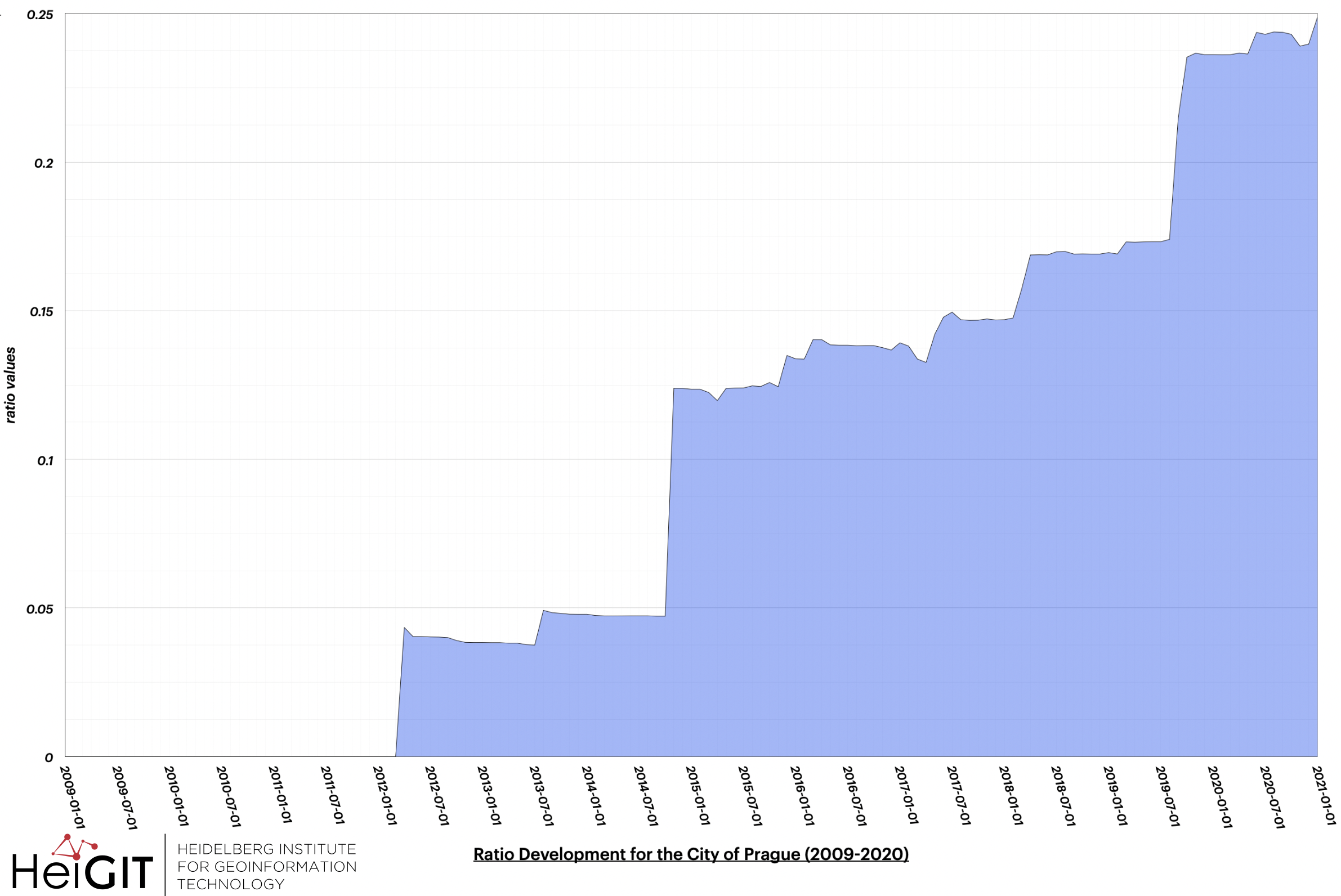
Although the ratio values increase over the years they barely reach 25%. When looking at the datasets we got from our requests, the part of the railway network which actually bares the information of the operator tag seems rather „up-to-date“ as even the name change of the Správa železnic in January 2020 was implemented rather quickly after coming into effect. Yet some of the railway network does not bare the information of an operator, although they most likely belong with one of the two main operators that were named in the dataset, namely Správa železnic & Dopravní podnik hlavního města Prahy, e.g. parts of the metro network do not have the operator tag. The exact reason for that appears to be unclear.
There is a whole list given when looking at the source tag in the full-history dataset, with a lot of them appearing to be linked to the Czech Office for Surveying, Mapping and Cadastre (ČÚZK for short) who offers quite a bit of GIS data. Interestingly enough the operator count wasn’t really used until January 1st, 2012. Throughout the years the overall trend of the ratio values is positive with a few data jumps. Since October 1st of 2016 the ČÚZK has been modifying and updating the INSPIRE-dataset which also happened in connection to their participation of the European Location Framework (ELF) project. The availability of the data might be related for the better ratio values by the end of the given timeframe.
Below you can see the output dataset of the full-history extraction with the Správa železnic operator data highlighted in magenta and the Dopravní podnik hlavního města Prahy operator data highlighted in yellow. The rest of the the railway network remains without an operator tag:
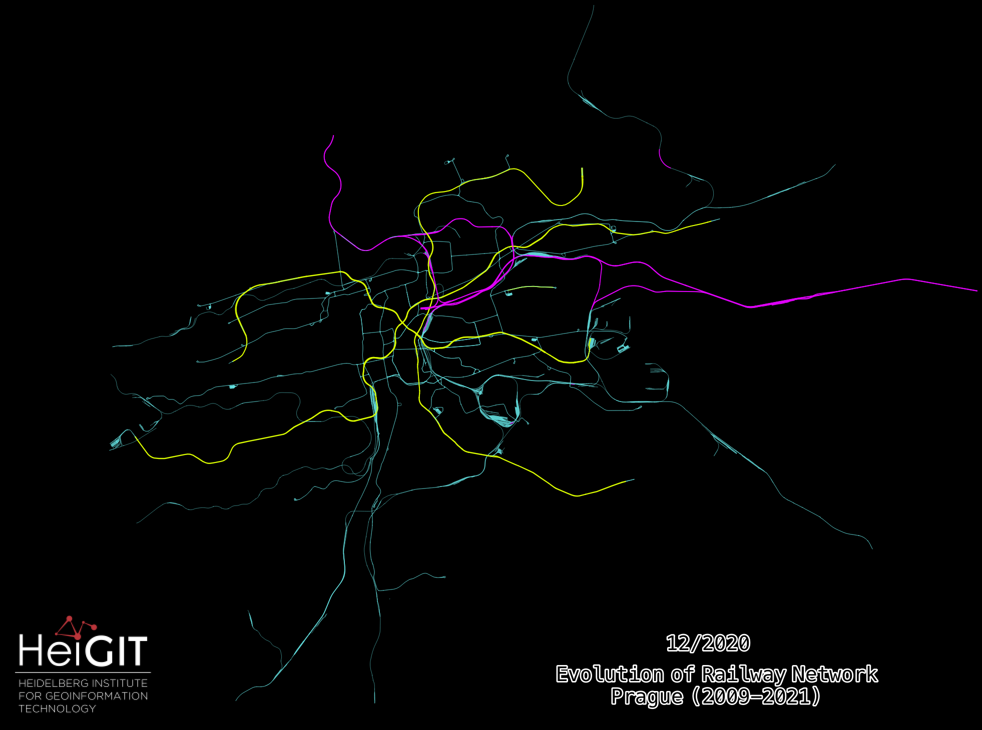
Interestingly enough most of the Metro Network (yellow highlighted lines) appears to be tagged with the operator information when looking at the picture. So at least the subway of Prague appears to have that tag added to it through the years. The “operator-less” part of the railway network however appears to be most of the cities tram network and only some parts of the railway=rail are tagged with operator information (highlighted in magenta).
Even though the ratio values itself are quite low, there is a lot of overall railway data given, especially at the beginning of the timeframe. When looking at the sources, it appears like there has been the opportunity to import data from e.g. orthophotos and datasets given by the Ústav pro hospodářskou úpravu lesů Brandýs nad Labem (ÚHÚL for short), so the Czech Forest Management Institute, or the ČÚZK. Furthermore, the source given for quite some data was Bing. So these input opportunities appear to be the reason why there is quite a lot data given from the start, but when taking the operator tag as our indicator of completeness into consideration, a great part of it appears to be incomplete for some reason. Note: the source=uhul:ortofoto is not being used anymore (since ~Summer 2015) but still had an impact on the dataset in the beginning of the timeframe looked at.
Conclusion:
At last, our region could ideally teach you how to animate a map yourself and has shown you an approach to a completeness analysis with a certain tag. Although the overall ratio values of the city of Prague are still quite small, the local mapping community appears to be rather motivated and active, so one can assume that there is a good chance for an operator tagged future for Prague.
Thank you for reading this months blogpost and stay tuned for there is more to come! As always, you can reach out to us via our email address ohsome(at)heigit(dot)org.
Background info: the aim of the ohsome OpenStreetMap History Data Analytics Platform is to make OpenStreetMap’s full-history data more easily accessible for various kinds of OSM data analytics tasks, such as data quality analysis, on a regional, country-wide, or global scale. The ohsome API is one of its components, providing free and easy access to some of the functionalities of the ohsome platform via HTTP requests. Some intro can be found here:
- ohsome general idea
- ohsome general architecture
- how to become ohsome blog series
- how spatial joins queries work in the OpenStreetMap History Database OSHDB