
Working with OpenStreetMap data is an exciting topic that often reveals astonishing insights. The free and open nature of the project allows a plethora of analyses topics. We at HeiGIT often concentrate on global quantitative analyses and visualisations powered by the ohsome framework. But our tools also enable you to gain more detailed, multifaceted or qualitative insights. However, before starting any investigation, one major question needs to be solved:
Which data should I include in my analyses?
Any object in OSM contains potentially viable information for any analyses because at least one person at one point of time decided it should be there. Currently the database contains more than 9 billion elements and it is growing (e.g. about 10% in the last year). But watch how that number will plunge to a manageable amount by applying a few simple filter steps. In the following we provide our personal defaults for reducing the overwhelmingly large OSM dataset into a meaningful chunk that should fit your interest very well.
- Visibility: Ignore deleted elements and elements without tags unless you really need them
- Keys: Start with the so-called “Map Features”
- Values: Prefer allowlists over blocklists over *
- Geometry: Choose reasonable geometry types that match the real-world objects you have in mind
- Area-of-interest: Avoid too simple and too complex bounding geometries
While OSM seems ubiquitous nowadays, hardly anybody uses all of OSM. This will be the key takeaway of our post: Everybody uses OpenStreetMap, no one uses the entire OpenStreetMap.
Note:
This guide is mostly suitable for all with basic GIS and OSM data knowledge.
All analyses presented were made for the data around the 2022-01-01. You can take a look at the code at https://gitlab.gistools.geog.uni-heidelberg.de/giscience/big-data/osm_data_basics_blogposts.
We want to emphasize that the following guidelines are no rules. We appreciate the freedom and possibilities for diversity of the project, yet have to make decisions in order to be able to handle the data.
Visibility: Ignore deleted elements and elements without tags unless you really need them
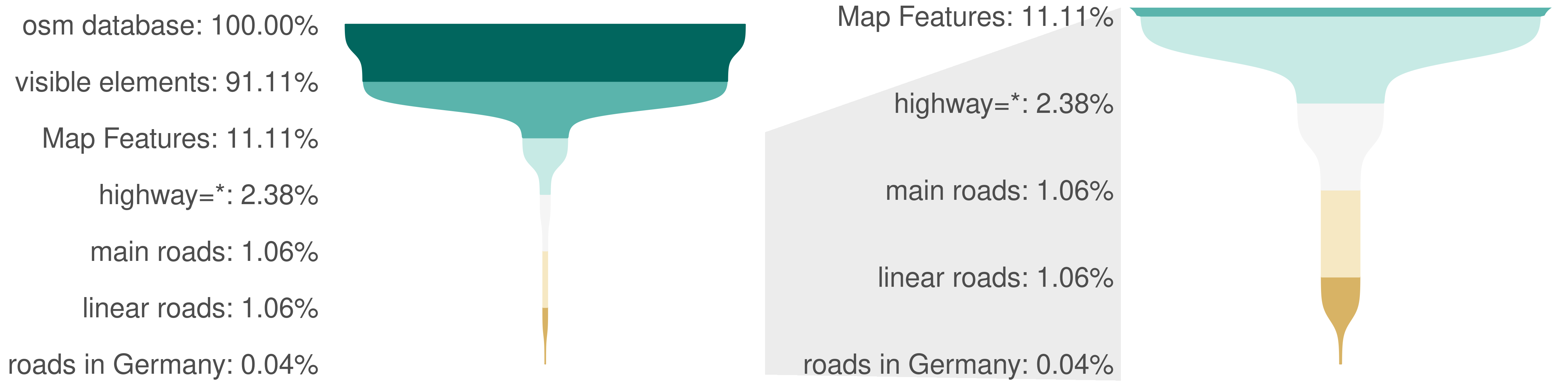
In most use cases you will not work with deleted elements or elements that do not carry any tags. Many OSM tools and also the ohsome framework implicitly encode these filters for you already, for a good reason. But we want to make you aware of them to highlight the size of the whole OSM data. Deletions are a relatively rare but possible action when contributing to OSM. Ignoring deleted objects reduces the number of OSM elements to around 8.2 billion.
The second, somehow hidden, filter again drastically reduces the number of potentially relevant elements to around 1 billion. This is achieved by ignoring elements without tags. Most of these elements with no tags are due to the OSM data schema that requires elements of lower dimension to create higher dimensional elements (e.g. points to create a line). These are not representing any real world objects or at least cannot be associated with any as it is completely unclear what that element is. They can (and will) be safely ignored in most cases as they bring no valuable information for further analyses.
Keys: Start with the so-called “Map Features”
Now that we have our set of elements that represent some ‘currently existing real world objects’, we can continue to extract the data for our analyses meaning the object types we are interested in. Object types are described by tags which are key=value combinations. To get started, we recommend to first select matching keys.
While of course this is not assured, keys often provide a reasonable grouping of objects. One attempt to foster coherence at the key-level are the so called ‘Map Features‘ which are a list of tags grouped by topic. The Map Features list currently contains 27 keys1 or object types. Examples are building=* or highway=*. Choose the primary keys that fit to your analyses and consider objects with multiple or no primary keys appropriately.
Following up from the ~1 billion non-deleted OSM elements with tags, filtering using the highway key gives us around 214 million remaining elements.
Values: Prefer an allowlist over a blocklist over *
The Map Features can then be subdivided by their value which can be thought of as the Map Feature Type. Examples are highway=motorway or highway=primary. In the next step we strongly advise to carefully hand select the Map Feature Types. While a wildcard selection of all values of a specific key is handy and blocklisting some undesired tags is possible, using an allowlist of selected tags has several advantages: Your analyses will be more comparable and stable over time, e.g. by preventing new tags to sneak into your data. A hand selected list of tags is also easier to report, maintain and investigate for error sources. We propose the following considerations how to select tags:
- How common is a tag?
- Is the tag documented?
Apart from the wiki, taginfo and taghistory can provide valuable information on how tags are actually used. Still the variety of values can be overwhelming including evolving tags, failed proposed tags, typos and the like. When looking at taginfo, the most common values are quickly found and will in most cases be relevant for you. You can ask yourself: If the tag is ignored, will there be a considerable total amount or fraction of the data removed? For instance you may consider that you already have >90% of all buildings when only selecting first three values (yes, house, residential). Any additional tag (e.g. garage, detached) will only add a small fraction of your existing selection.
If you need to include tags in your analysis that are not common, the documentation of a tag can be a strong hint as to if, how and where a tag is used or if it is deprecated. Some tags may not be clearly defined and used in contradicting or diverse manners. Nevertheless, a thorough understanding of your data region is very important for this task. E. g. up until 2020-06-28 ‘landuse=raceway’ covered quite a large area in the Rhein-Neckar-Region even though only 26 objects of that type exist globally2.
Our funnel will continue with the following common and documented highway tags that we believe best represent the general street network:
- motorway
- motorway_link
- trunk
- trunk_link
- primary
- primary_link
- secondary
- secondary_link
- tertiary
- tertiary_link
- unclassified
- residential
This reduces the number of elements to 95.46 million.
Geometry: Choose reasonable geometry types that match the real-world objects you have in mind
Because the use of specific tags is not limited to a certain geometry type, we might still struggle to make sense of all the points, lines and polygons in our selection. Fortunately, with the ohsome framework, you don’t have to worry too much about this. We advise you to hand select the valid geometry types to filter the elements you want to consider. In most cases the geometry type will be defined by your analysis question. In case of doubt, you can always consult the OSM wiki. Another option is to run a preliminary data analyses to get an overview on the geometry types of the selected elements in your study region.
For our use case of analysing the length of the general street network, considering only elements with the geometry type “line” seems appropriate. This gives us a final set of 95.43 million elements globally and we can now create meaningful and interesting analyses on any data insight we need!
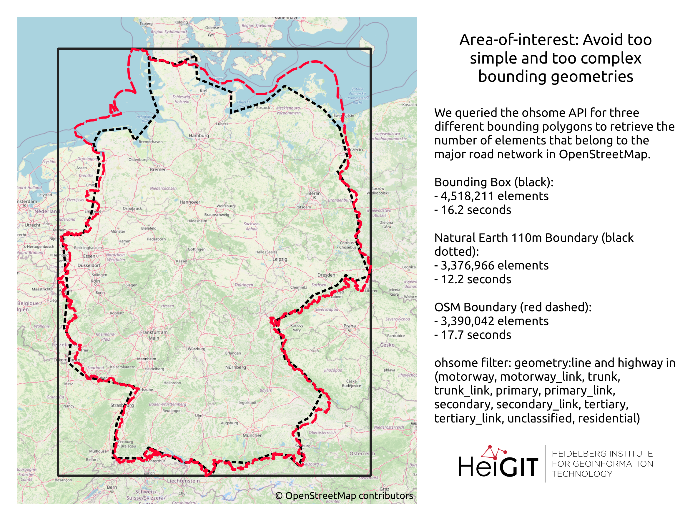
Area-of-interest: Avoid too simple and too complex bounding geometries
For a global data overview as we presented here, the analyses region is immutable, but in most cases the region of interest is bound to a much smaller area. Therefore it has to be emphasized again that mapping in OSM can differ for the same elements between regions which should be taken into account, either when running the analyses or when interpreting the results.
We recommend that, before running your query, you may simplify your area of interest. The more complex your geometry(s), the more computation is needed to construct and check geometric computations like intersections or aggregation by area. This will help to speed up your query and make the results more comparable. The problem of too complex area-of-interest polygons often arises when analysing data at the country level. As a rule of thumb you can assume that the larger the size of your area-of-interest, the lower the resolution of your boundaries should be.
The most simple geometry would of course be a bounding box. But this may not well cover your area especially if it is very large and earth curvature becomes an influence. The next best choice is therefore a convex polygon. For country boundaries you should consider using a simplified geometry, e.g. as provided by Natural Earth Data. When working with boundaries obtained from OSM you should consider running a cartographic generalization, e.g. in QGIS. A more detailed outline with more vertices and holes should only be used, if that level of detail is necessary.
Conclusion
And there you are, equipped with all basic information to get started on OSM data filtering. All in all the advice comes down to ‘Be as specific as possible’ but of course that can be a complex task where no universal guideline is available. Yet we hope that this post will contribute to more uniform and comparable analyses, we certainly will try to adhere to these standards for our own analyses. If you found this post useful stay tuned for our next post in the series on the basics of OSM data handeling.
Further readings:
- OSM basics blog series
- How to become ohsome blog series
—
1We will talk about that list in detail in a future blog post in this series.
2This is in fact a good example where the count of objects is not the main interest but rather the area covered and the development over time, a topic that is also coming up.